Skip to content

Operations

Averages do not show where the model starts to fail

In the series of posts so far, I have shown you how selecting models for a portfolio is more nuanced than choosing the top model with the lowest mean absolute error. There is one more thing left: robustness.

A model must perform well on average. However, in the cases where it is underperforming, it should not be too much worse. Average scores or metrics hide these details. They are necessary — but they do not tell the complete story.

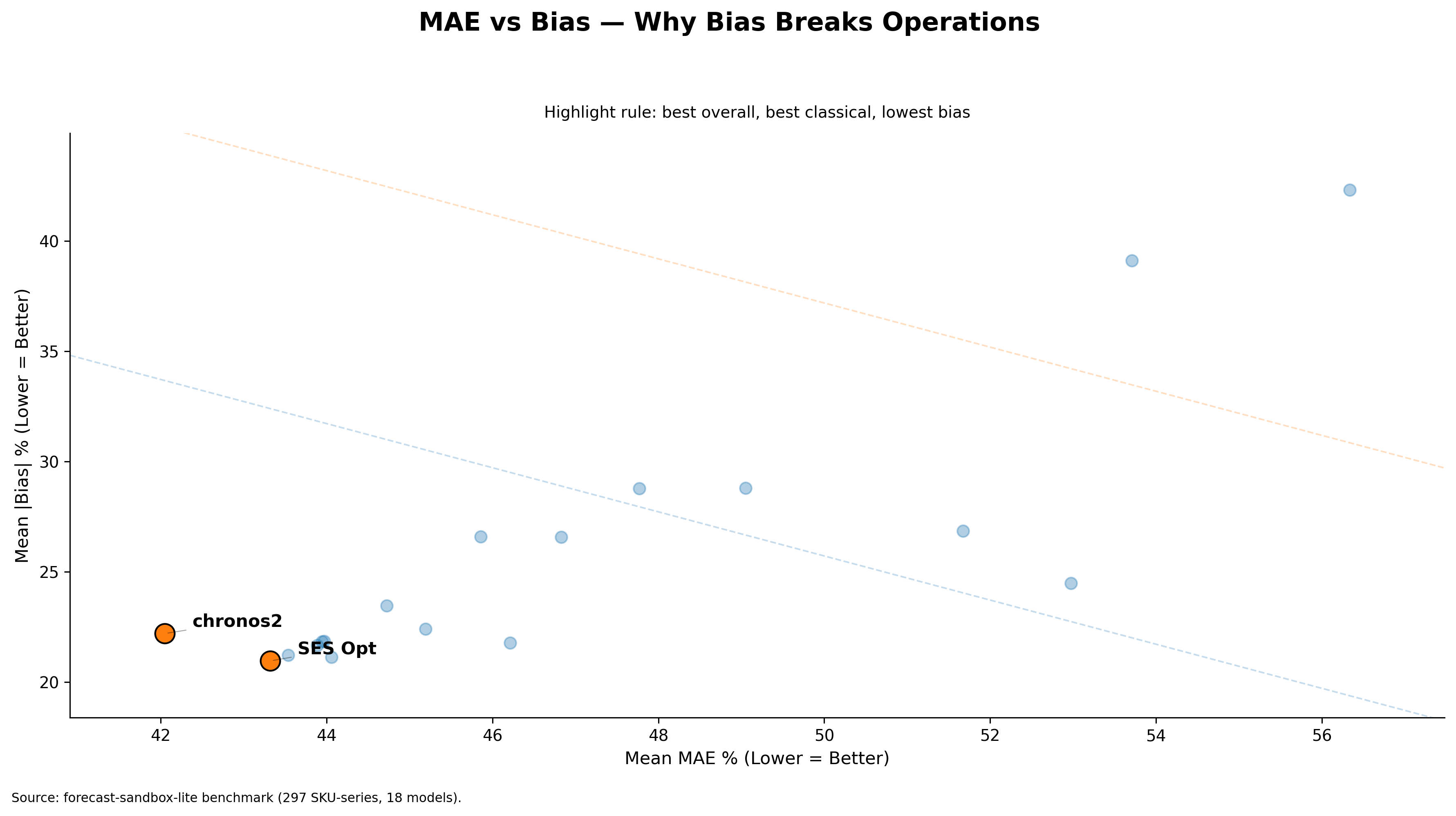
In my benchmark, Chronos2 had the lowest mean score (MAE% + Bias%) of 64.25, followed by SES Opt at 64.28. On average, they are nearly equal in performance.

When a worse case appears in demand forecasting, the model should not produce results that are too far off. Take a large supermarket as an example. As its operator, you would not want a model that performs well on lower-margin items but fails on higher-margin ones. This is what needs to be checked before deploying a model in production for demand forecasting.

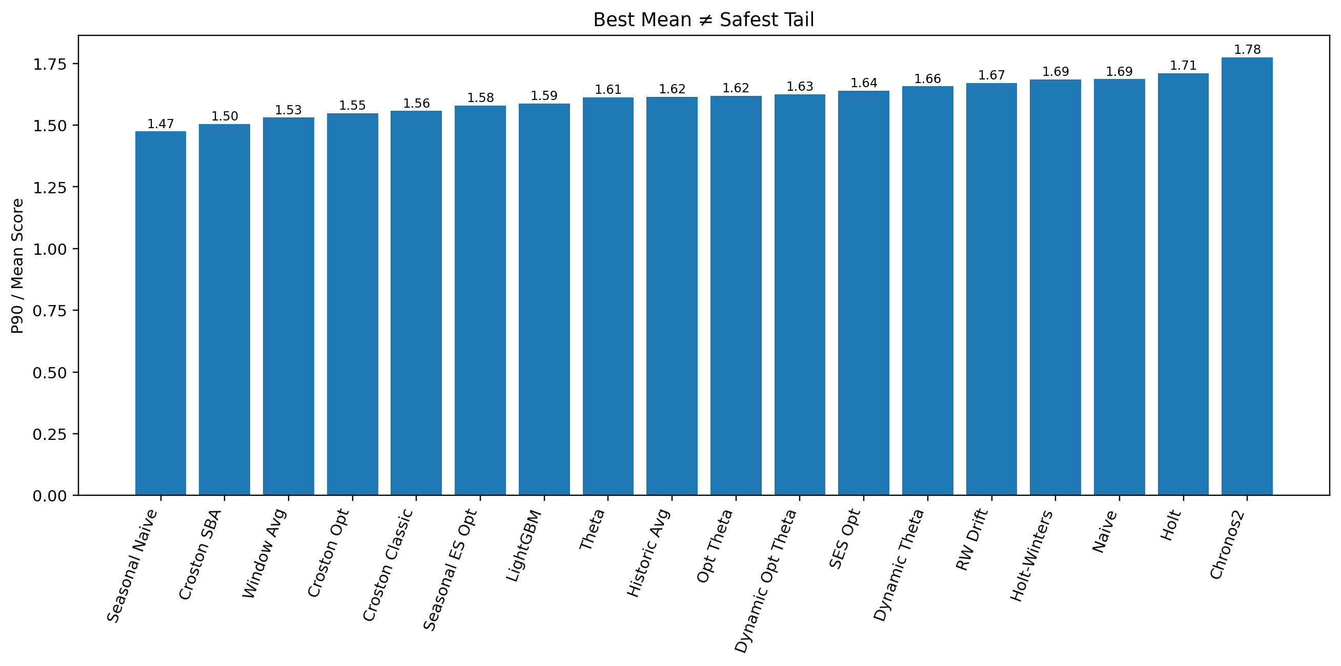
There is a straightforward way to make this visible. Look into percentile performance — specifically the P90 of the score, which shows performance at the bad tail of the portfolio. Then compare it to average performance (mean). Simply calculate P90 / Mean to check how robust a model is relative to others. A lower ratio means the model stays more controlled. A higher ratio means it deteriorates more sharply. This is not a complete framework for risk assessment, but it is a good start.

Average score puts Chronos2 at the top. However, in previous posts I already showed that SES Opt carries lower absolute bias than Chronos2. Now let us add this new layer to the comparison.

Model Mean Score Bias P90 Score P90 / Mean
Chronos2 64.25 22.20 114.07 1.78
SES Opt 64.28 20.96 105.36 1.64

SES Opt now looks more deployable — near-top average performance, lower bias, and more controlled weakening once performance moves into the bad tail.

The plot below shows that Chronos2 has the worst tail behavior among all models benchmarked, while SES Opt is far more stable where it matters.

Tail Risk Ratio across models

Tail behavior becomes especially important when:

  • Forecast misses are costly
  • Planners remember bad cases more than average performance
  • Unstable behavior weakens trust in the system
  • A default model is expected to remain dependable across the full portfolio

The larger argument is this: average scores do not ensure operational trustworthiness. One needs to combine all metrics — MAE%, Absolute Bias%, MAE% + Absolute Bias%, and P90 / Mean — to arrive at the right decision.

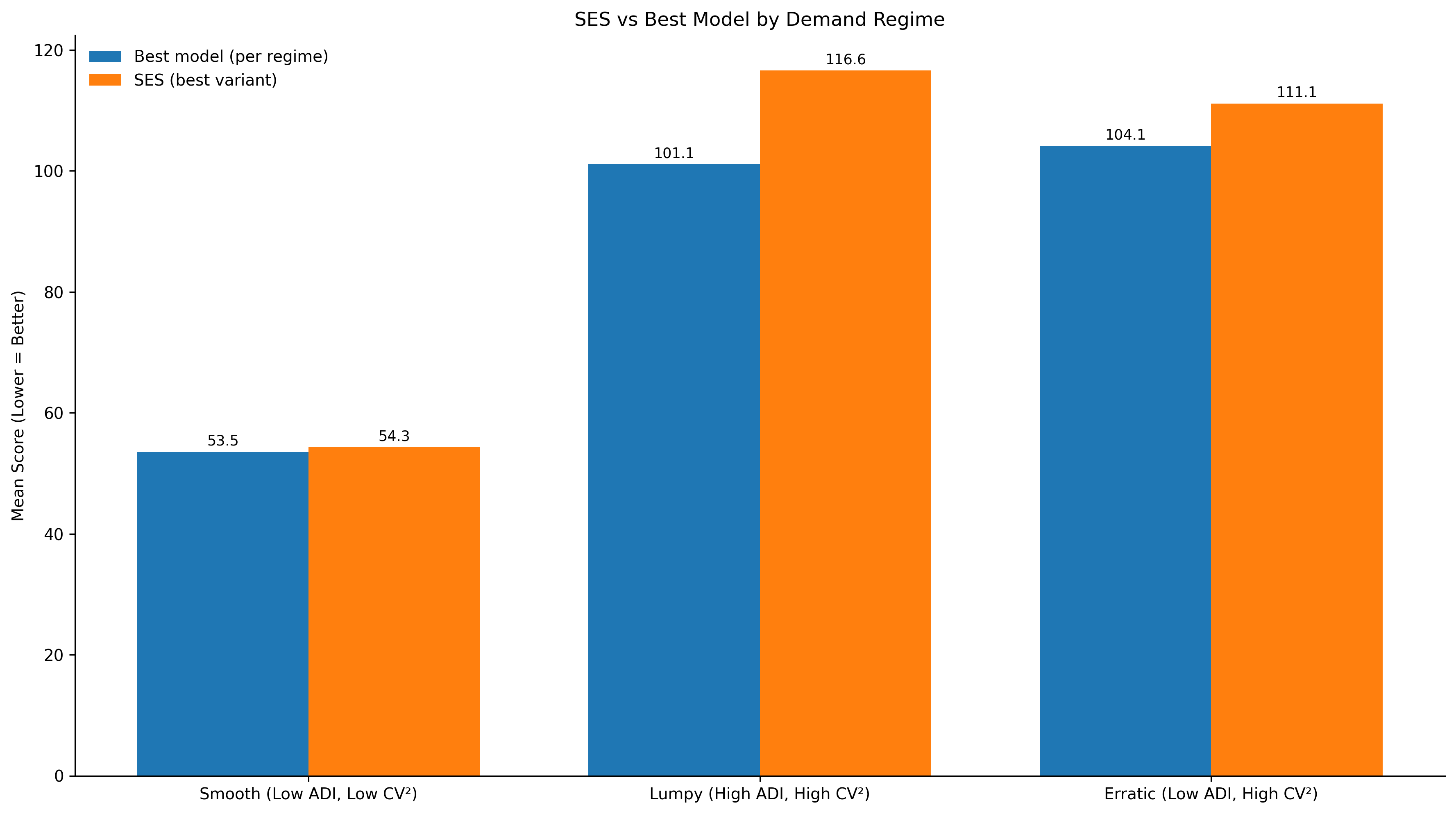
Note: This article does not argue that average metrics are unnecessary or that there is no need for regime-aware forecasting.

There is no best forecasting model without a demand regime lens

in Demand Forecasting, Model-Selection, Operations · 5 min read


A portfolio-level benchmark creates a real temptation. Rank the models, pick the strongest overall performer, and standardise on it. That choice is a good start — it reduces complexity, simplifies explanation, lowers governance overhead, and makes deployment and maintenance easier. In practice, that is often how model policy begins.

Starting there is not an issue. Staying there is.

There are different underlying demand structures in a portfolio and they put different demands on the model being built for it. If a portfolio model is chosen globally, it may end up partially optimised for the demand structure that is most frequently present — and underperform everywhere else.

Take a supermarket that sells everything from daily household needs to high-end computing devices. The margins on day-to-day needs may not be high, but high footfall and sheer volume keeps the operation running. However, it may also be important to focus on products that are luxury and sold infrequently — MacBook Pros, luxury dresses, perfumes etc. Here the market can make higher margins if it is able to plan more appropriately for demand. That is, if the supermarket can supply for demand in such a way that sunk costs are low and demand is met better, the market makes more margins on those products.

In plain terms: forecasting of each product does not carry equal cost, margins, and demand structure. A forecasting portfolio cannot treat all products as equal weights. This is where demand regimes become critical.

The global ranking compresses different demand structures into one number. It is only when the portfolio is segmented that the cost of that assumption becomes visible.

In the last post, we saw that SES performed nearly as well as the best model in smooth demand — but its performance suffered in other demand types. Once the first model starts performing well, one needs to pivot toward the second set of larger gains — which come from increasing complexity only a little by using models suited to each demand structure. I studied the best performing model per regime to make this concrete.

Top 5 models by demand regime — smooth, erratic, lumpy. Lower score is better. 
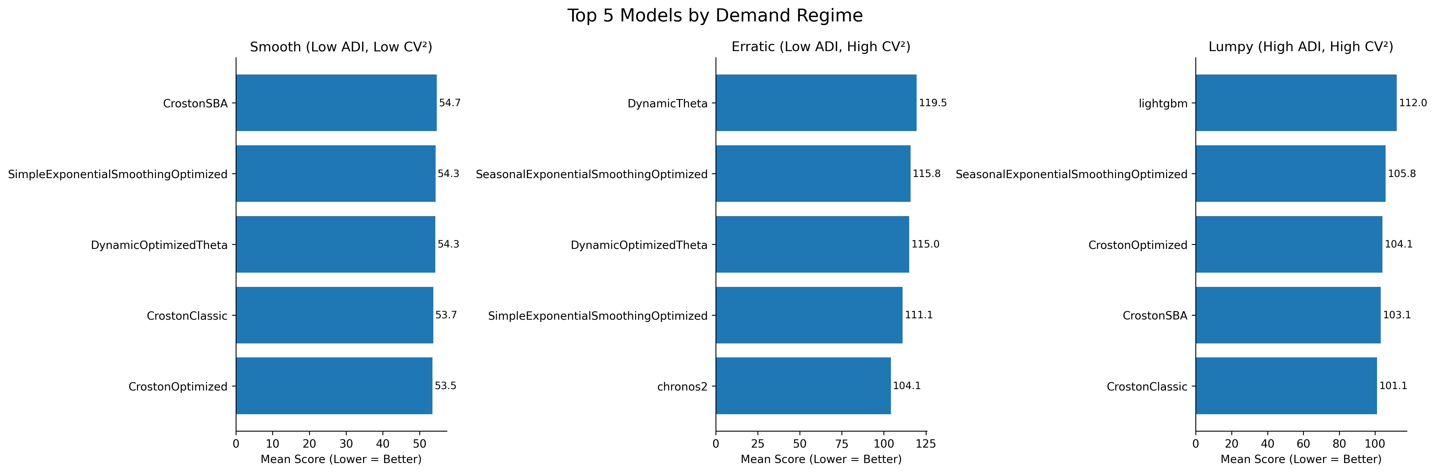
Top 5 models per regime — smooth, erratic, lumpy. Lower score is better.

In smooth demand, CrostonOptimized was the top model with the lowest score. The top five models were neck and neck in competition — the spread between them was small.

As soon as we shift to erratic demand, the best model was Chronos2 — and this time with a wider range of score differences between the top model and the rest.

In lumpy demand, CrostonClassic came out on top.

This underlines the point. The model chosen as the best portfolio model — SES Optimized — was not the top model in any of the demand regimes. It was consistently among the top performing models across regimes, but had significant deviations from the top model in each one. A globally competitive model is not automatically the best choice for the demand structures that matter most operationally.


A note on scope. These results are specific to this dataset — a daily, perishable, intermittent-demand retail context using 18 univariate models on a 297-SKU subset.

The transferable insight is not that one named model will always win a given regime in every domain. It is that model rankings can change materially once demand structure is separated instead of averaged together.


Model choice should follow demand structure — not hype toward newer models, and not habit toward familiar ones. A small tradeoff in complexity can unlock meaningfully better results.


Benchmark: 297 SKUs · FreshRetailNet-50K · 18 univariate models · Daily perishable retail data · ADI/CV² segmentation · Lower score = better forecast accuracy. Regime-level results; individual SKU variance exists within each category.

Simple models remain operationally viable — until demand stops being smooth

in Notes, Forecasting, Operations · 6 min read


In previous posts, I showed how simple models like SES Optimized are still performant and may give better results than other univariate models. At portfolio level they can perform well. However, choosing a single model without considering demand structure means not capturing the full benefit of these models.


What forecasting models are for

Forecasting models are not made for getting benchmark scores on a portfolio.

They are used to make better decisions for replenishment, purchasing, inventory positioning, working capital allocation, and service-level stability.

Global use of one model is enticing to the practitioner. It reduces complexity. It simplifies explanation. It lowers governance overhead. It makes deployment and maintenance easier.

However, this decision comes with a cost — non-performance across different types of demand.

A model may look strong at the overall portfolio level and still be a weak default for large parts of it.


Demand is not uniform

Demand patterns are not the same across a portfolio. A portfolio generally contains fundamentally different underlying demand patterns — smooth, erratic, intermittent, and lumpy. Each makes different demands on forecasting models.

A commonly used framework to classify such patterns is the ADI/CV² framework. It checks two things: how frequently demand occurs, and how variable it is when it occurs.

Most portfolios contain all regimes simultaneously. A model that performs well in one regime may not perform well in others. Most forecasting policies do not account for this — they try to minimise the number of models used instead.

SES Optimized is a recency-based model. It performs reasonably well when the underlying signal is stable. In such cases, recent history still carries meaningful information about the near future. The model is simple, efficient, and often surprisingly competitive.

However, if the signal is not inherently stable, recency does not carry as much information about the upcoming future — and performance degrades.


The benchmark

To make this concrete, I benchmarked 18 univariate forecasting models on a 297-SKU subset from FreshRetailNet-50K and grouped SKUs using the ADI/CV² regime lens. Lower score is better.

SES Vs Best Model Per Regime

Above plots the performance of SES Optimized against the best performing model in each regime. The gap is the performance cost of holding SES as the default across that regime.

Demand regime Best model score SES score Gap
Smooth 53.5 54.3 0.8
Erratic 104.1 111.1 7.0
Lumpy 101.1 116.6 15.5

The gap is the performance cost of holding SES as the default across that regime.

In smooth demand, SES Optimized remains very close to the best performing model. As soon as it moves into erratic and lumpy demand, it is no longer the optimal default.

What this shows. Without the regime analysis, one would likely choose SES Optimized as the single operational default — it performs well at portfolio level. The demand-based analysis shows exactly where this model holds and where it fails.

A note on scope. These results are specific to this dataset — a daily, perishable, intermittent-demand context. SES being competitive in smooth demand here does not mean it will be competitive in smooth demand on a different dataset, a different category, or a different operating context. The regime lens is the transferable insight. The specific numbers are not.


What this means in practice

Regime Verdict
Smooth SES is defensible here. Governance simplicity earns the marginal accuracy concession.
Erratic SES is no longer optimal. Stronger alternatives are worth evaluating.
Lumpy SES is not a sound default. The performance cost is too large to absorb.

Make the model policy as simple as possible — but not simpler than the demand structure allows.

That said, this is not always a day-one decision. Regime-aware model selection requires data infrastructure, classification logic, and governance for multiple model types. That cost is real.

For many organisations, the right first move is still a simple model deployed globally — not because it is optimal across all regimes, but because getting it running cleanly, with proper monitoring and bias tracking, is already a meaningful operational capability. It is the foundation that makes the next step possible.

The regime analysis then becomes the natural next question: now that we have a baseline, where is it costing us? That is a better question to ask from a position of operational stability than from the start of a forecasting programme.

Simple models are not the final destination. But for many teams, they are the right place to begin — and understanding exactly where they hold is what makes the transition to regime-aware policy a deliberate step rather than a reactive one.


Model choice should follow demand structure — not hype toward newer models, and not habit toward familiar ones.

That is what separates a model that looks good in a benchmark from a policy that performs well in a real portfolio.


Benchmark: 297 SKUs · FreshRetailNet-50K · 18 univariate models · Daily perishable retail data · ADI/CV² segmentation · Lower score = better forecast accuracy. Regime-level results; individual SKU variance exists within each category.

Your best forecast model might be your biggest operational risk

Forecasts are not made to win benchmarks. They are made for decision-making.

Running a business means dealing with volatility, especially in demand and supply. The better a business can estimate future demand, the better it can plan inventory, negotiate procurement, allocate working capital, and maintain service levels. Better forecasts do not remove uncertainty. They enable better decisions under uncertainty.

Better estimation of demand means that a large chunk of inventory decisions is made far ahead of time. That improves purchasing, product availability, customer satisfaction, and the cost of understocking or overstocking. In that sense, forecasting is not just a modeling problem. It is a business control system.

Due to the inherent volatility of the world, even great forecasts are meaningfully off. Most forecast models are optimized to reduce the gap between forecast and reality without caring about direction. That is what absolute error captures: how far you were from reality, regardless of whether you were too high or too low.

Direction, however, matters over an operational horizon.

That is what bias captures: whether a forecasting system consistently leans in one direction over time. A system that consistently over-forecasts creates one kind of operational damage. A system that consistently under-forecasts creates another. In both cases, the damage compounds quietly.

For any given horizon, two numbers define forecast performance:

  • MAE % — how wrong you are on average, in magnitude
  • Average Bias — how wrong your system has become, directionally

MAE tells you how wrong you are. Bias tells you how wrong your system has become.

Both metrics are important. But they operate on different timescales and carry different risk profiles. MAE reflects day-to-day noise. Bias reflects directional drift — systematic error. A business can often absorb more day-to-day fluctuation. But bias becomes visible only after the damage is done. A model that is marginally worse on MAE but holds lower bias can still be the stronger operational choice.

The right operating lens is two-dimensional — not a single leaderboard number.

To make this concrete, I benchmarked 18 univariate forecasting models on a 297-SKU subset from FreshRetailNet-50K: daily retail data, intermittent demand, perishable operating context.

Executive view

The executive view makes the tradeoff visible immediately: Chronos2 leads on MAE %, while SES Opt holds lower absolute bias.

Executive view: MAE vs Bias

Two models ended up very close:

Model MAE % |Bias| % Composite Score
Chronos2 42.05 22.20 64.25
SES Opt 43.32 20.96 64.28

This was much more nuanced than a simple Foundation Model (Chronos2) vs Classical Model (SES Opt) story.

Chronos2 leads on MAE % by 1.27 points, or roughly 2.9%.
SES Opt leads on absolute bias by 1.24 points, which means about 5.6% less directional drift.
On composite score, they are essentially tied: 64.25 vs 64.28.

That is the real lesson.

If you optimize only for MAE, you would likely pick Chronos2. But that decision also comes with higher directional drift. Over time, that drift can become slow-motion inventory distortion — the kind that often does not show up in a standard forecasting review until it has already become a business problem.

So the better question is not:

Which model has the lowest error?

The better question is:

Which model gives acceptable error with the least directional risk?

That question should change model selection.

Operational excellence is not achieved by minimizing forecast error alone. It is achieved by jointly managing error magnitude and directional drift — and by making both visible in the decision process.

A model with slightly better headline accuracy can still be the weaker operational choice if its bias is allowed to accumulate unchecked.

Technical view

The full benchmark view shows that this is not a cherry-picked comparison. The Chronos2 vs SES Opt tradeoff sits inside a broader portfolio of 18 evaluated models.

Technical view: MAE vs Bias

That is why the best forecast model on paper can still be your biggest operational risk.